Quantcast
Channel: FlexMonkey
Viewing all 257 articles
Browse latest View live

Histogram Equalisation with Metal Performance Shaders

$
0
0


Histogram equalisation is a quick way to enhance contrast and bring out detail in an otherwise flat image by both stretching and flattening an image's histogram. The operation is available in both vImage and Metal Performance Shaders (MPS). The technique for the latter is a little bit tricky, so this post demonstrates how to execute an equalisation using MPS with a little companion project

Histogram Equalisation in Practice

Given this rather flat image of some clouds with the majority of pixels are bunched towards lighter tones:


Equalising the histogram evens out the tonal distribution across the entire available range and flattens the curve slightly. 


Implementing with Metal Performance Shaders

Our first step is some basic setup: we need a device, which is the interface to the GPU, and a command queue and command buffer:

        let device = MTLCreateSystemDefaultDevice()!
        let commandQueue = device.newCommandQueue()
        let commandBuffer = commandQueue.commandBuffer()

If our source image of the clouds, inputImage, is provided as a CIImage, our next step is the create a Metal texture that represents it. We can do this by creating a Core Image context that uses the Metal device and calling its render function to draw to a texture created by the device:

        let textureDescriptor = MTLTextureDescriptor.texture2DDescriptorWithPixelFormat(
            .RGBA8Unorm,
            width: Int(inputImage.extent.width),
            height: Int(inputImage.extent.height),
            mipmapped: false)
        
        let colorSpace = CGColorSpaceCreateDeviceRGB()!
        
        let inputTexture = device.newTextureWithDescriptor(textureDescriptor)
        let destinationTexture = device.newTextureWithDescriptor(textureDescriptor)
        
        let ciContext = CIContext(MTLDevice: device)
        
        ciContext.render(
            inputImage,
            toMTLTexture: inputTexture,
            commandBuffer: commandBuffer,
            bounds: inputImage.extent,
            colorSpace: colorSpace)

Now to start the equalisation process. We need to calculate the histogram of inputImage. MPSImageHistogram requires an empty MPSImageHistogramInfo instance:

        var histogramInfo = MPSImageHistogramInfo(
            numberOfHistogramEntries: 256,
            histogramForAlpha: true,
            minPixelValue: vector_float4(0,0,0,0),
            maxPixelValue: vector_float4(1,1,1,1)) 
        
        let calculation = MPSImageHistogram(
            device: device,
            histogramInfo: &histogramInfo)

The histogram info object is wrapped in a Metal buffer and the MPSImageHistogram can be encoded to the command buffer:

        let histogramInfoBuffer = device.newBufferWithBytes(
            &histogramInfo,
            length: sizeofValue(histogramInfo),
            options: MTLResourceOptions.CPUCacheModeDefaultCache)
        
        calculation.encodeToCommandBuffer(
            commandBuffer,
            sourceTexture: inputTexture,
            histogram: histogramInfoBuffer,
            histogramOffset: 0)

Now that the MPSImageHistogramInfo is populated with the image's histogram, it can be equalised. The histogram info object used to instantiate an MPSImageHistogramEqualization which has its transform function encoded to the command buffer before being encoded itself:

        let equalization = MPSImageHistogramEqualization(
            device: device,
            histogramInfo: &histogramInfo)
        
        equalization.encodeTransformToCommandBuffer(
            commandBuffer,
            sourceTexture: inputTexture,
            histogram: histogramInfoBuffer,
            histogramOffset: 0)
        
        equalization.encodeToCommandBuffer(
            commandBuffer,
            sourceTexture: inputTexture,
            destinationTexture: destinationTexture)

The final step is to commit the command buffer for execution on the GPU:

        commandBuffer.commit()

The final target texture is destinationTexture which can be converted to a CIImage for display with the init(MTLTexture:options) initialiser:

        let ciImage = CIImage(
            MTLTexture: destinationTexture,
            options: [kCIImageColorSpace: colorSpace])

Easy! 

The Accelerate v/Image Alternative

You may decide to plump for vImage which does it in one step:

        vImageEqualization_ARGB8888(
            &imageBuffer,
            &outBuffer,
            UInt32(kvImageNoFlags))

Equalisation versus Contrast Stretch

Sadly, Metal Performance Shaders doesn't include contrast stretch. Contrast stretch is not dissimilar to equalisation, but doesn't attempt to flatten the curve shape, it simply stretches it to the full value range. vImage, however, does include contrast stretching. Here's a vImage equalisation (pretty much identical to its MPS equivalent):


...and here's vImage contrast stretching:


Although Core Image doesn't have these histogram operations, it can go some way to mimicking them with the tone curve filter generated by auto adjustment filters:

        guardlet filter = inputImage
            .autoAdjustmentFiltersWithOptions(nil)
            .filter({ $0.name == "CIToneCurve"})
            .firstelse
        {
            return
        }
        
        filter.setValue(inputImage, forKey: kCIInputImageKey)

Which yields:

Core Image for Swift 

Version 1.3 of my book, Core Image for Swift, is due out very shortly which explores histogram operations with vImage in more detail.

Core Image for Swift is available from both Apple's iBooks Store or, as a PDF, from Gumroad. IMHO, the iBooks version is better, especially as it contains video assets which the PDF version doesn't.


Nodality for AudioKit: Node Based Synth for iPad

$
0
0


I've done a fair bit of tinkering with the amazing AudioKit framework and I've also done a fair bit of tinkering with node based user interfaces. Ever since AudioKit introduced nodes, I've been planning to marry the two together and build Nodality for AudioKit. I'm pleased to say after only a few days of work, it's working, stable, open-sourced and available here.

I actually open-sourced the node based user interface component back in September 2015 (see: A Swift Node Based User Interface Component for iOS), so I dusted it off and got cracking. 

AudioKit's new API makes building networks of nodes super simple. Let's imagine some crazy system with a pink noise source passing though a reverb which is mixed with a square wave oscillator. The network could look a little like this:


The code required to build this network is simply:

        let pinkNoise = AKPinkNoise()
        let reverb = AKReverb(pinkNoise)
        let squareWave = AKSquareWaveOscillator()
        let dryWetMixer = AKDryWetMixer(reverb, squareWave, balance: 0.5)
        
        pinkNoise.start()
        squareWave.start()
        
        AudioKit.output = dryWetMixer

        AudioKit.start()

Take a look at the video above to see the interaction design:

  • To create a new node, do a long press on the background. A modal form sheet will pop up allowing the selection of the type of the new node.
  • To create a relationship between two nodes, long press on the source node. The screen background will turn to a light grey color and a further tap on the row of a target node will create the relationship. Illegal targets (e.g. attempting to create a relationship between a numeric node and an AudioKit node input) are greyed out.

A big shout out to Aurelius and Matthew who provided technical and moral support while I wrote this and to the rest of the AudioKit team for creating such an awesome framework. I know nothing about audio at all, and AudioKit has enabled me to write a node based synthesiser in a few days! 

Core Image for Swift Version 1.3

$
0
0


I'm pleased to announce that version 1.3 of my book, Core Image for Swift, is now available through Apple's iBooks Store and, as a PDF, through Gumroad

The main change is a new chapter discussing vImage - the image processing component of Accelerate. I focus mainly on the histogram and morphology functions: what they offer that "vanilla" Core Image lacks and how to integrate them in a Core Image workflow. Operations such as histogram stretching and equalisation are fantastically powerful tools and the new version of the book includes plenty of content explaining how they work and what they can do. 

If you'd prefer to see and hear me ramble on about image processing, above is a video of me talking about Core Image at a recent NSLondon

I'd suggest the iBooks version which includes video assets that the PDF version lacks.


Random Numbers in Core Image Kernel Language

$
0
0

I added a new Scatter filter to Filterpedia yesterday. The filter mimics the effect of textured glass with a kernel that randomly offsets its sample coordinates based on a noise texture created with a CIRandomGenerator filter. Because the Core Image kernel for this filter needs to sample the noise texture to calculate an offset, it can't be implemented as a CIWarpKernel, it has to be the general version: a CIKernel

A warp kernel is the ideal solution for this, but "out-of-the-box" Core Image Kernel Language doesn't support any of the GLSL noise functions. A quick bit of surfing led me to this super simple pseudo random number generator over at Shadertoy

We can see it in action by creating a quick color kernel:


    let colorKernel = CIColorKernel(string:
        "float noise(vec2 co)" +
        "{ " +
        "    vec2 seed = vec2(sin(co.x), cos(co.y)); " +
        "    return fract(sin(dot(seed ,vec2(12.9898,78.233))) * 43758.5453); " +
        "} " +

        "kernel vec4 noiseField()" +
        "{" +
        "  float color = noise(destCoord());" +
        "  return vec4(color, color, color, 1.0); " +
        "}")

Applying the kernel:


    let extent = CGRect(x: 0, y: 0, width: 2048, height: 480)
    let noiseField = colorKernel?.applyWithExtent(extent, arguments: nil)

Produces an even noise image:


I found passing in the destCoord() directly into the calculation produced some repetition artefacts; adding the additional line to generate seed eliminates those.

Implementing the pseudo random number generator in a warp kernel to produce the scattering effect is a simple step:


    let kernel = CIWarpKernel(string:
        "float noise(vec2 co)" +
        "{ " +
        "    vec2 seed = vec2(sin(co.x), cos(co.y)); " +
        "    return fract(sin(dot(seed ,vec2(12.9898,78.233))) * 43758.5453); " +
        "} " +
            
        "kernel vec2 warpKernel(float radius)" +
        "{" +
        "  float offsetX = radius * (-1.0 + noise(destCoord()) * 2.0); " +
        "  float offsetY = radius * (-1.0 + noise(destCoord().yx) * 2.0); " +
        "  return vec2(destCoord().x + offsetX, destCoord().y + offsetY); " +
        "}"
    )

This kernel uses the coordinates of the pixel currently being calculated (destCoord()) to generate two random numbers in the range -1 through +1 multiplied by a radius argument. The return value of a warp kernel is a two component vector that specifies the coordinates in the source image that the current pixel in the destination image should sample from. Given a radius of 40 against a 640 x 640 image of the Mona Lisa, we get:


The killer question is, how much faster is this warp kernel implementation over my original general kernel version - especially considering the latter also has additional filters for generating the noise and I've added a Gaussian blur for optional smoothing. 

Well, the answer is the warp kernel implementation is actually a tiny bit slower! A small refactor to inline the random number generation and only call destCoord() once gives the warp kernel version a very slight edge in performance (at the expense of elegance):


    let kernel = CIWarpKernel(string:
        "kernel vec2 scatter(float radius)" +
        "{" +
        "    vec2 d = destCoord(); " +
        "    vec2 seed1 = vec2(sin(d.x), cos(d.y)); " +
        "    float rnd1 = fract(sin(dot(seed1 ,vec2(12.9898,78.233))) * 43758.5453); " +
        "    vec2 seed2 = vec2(sin(d.y), cos(d.x)); " +
        "    float rnd2 = fract(sin(dot(seed2 ,vec2(12.9898,78.233))) * 43758.5453); " +
        
        "  float offsetX = radius * (-1.0 + rnd1 * 2.0); " +
        "  float offsetY = radius * (-1.0 + rnd2 * 2.0); " +
        "  return vec2(destCoord().x + offsetX, destCoord().y + offsetY); " +
        "}"


Core Image for Swift

The code for both versions of this scatter filter are available here. However, if you'd like to learn more about writing custom Core Image kernels with Core Image Kernel Language, may I recommend my book, Core Image for Swift.

Core Image for Swift is available from both Apple's iBooks Store or, as a PDF, from Gumroad. IMHO, the iBooks version is better, especially as it contains video assets which the PDF version doesn't.


A Core Image Transverse Chromatic Aberration Filter in Swift

$
0
0

Transverse or lateral chromatic aberration is an optical artefact caused by different wavelengths of light focussing at different positions on a camera's focal plane. It appears as blue and purple fringing which increases towards the edge of an image. In addition to the Wikipedia entry on chromatic aberration, there's a great article here at Photography Life which discusses the phenomenon in great detail.

Although the bane of many photographers, I've created a Core Image filter to simulate the effect which can be used to add a low-fi, grungy look to images. The basic mechanics of the filter are pretty simple: it essentially consists of three zoom filters each with a slightly different offsets for red, green and blue. The technique borrows from Session 515: Developing Core Image Filters for iOS talk at WWDC 2014. 

Let's look at the general kernel I've written for the filter and then step through it line by line:


    let transverseChromaticAberrationKernel = CIKernel(string:
        "kernel vec4 chromaticAberrationFunction(sampler image, vec2 size, float sampleCount, float start, float blur) {" +
        "  int sampleCountInt = int(floor(sampleCount));" + // 1
        "  vec4 accumulator = vec4(0.0);"// 2
        "  vec2 dc = destCoord(); "// 3
        "  float normalisedValue = length(((dc / size) - 0.5) * 2.0);" + // 4
        "  float strength = clamp((normalisedValue - start) * (1.0 / (1.0 - start)), 0.0, 1.0); " + // 5
        
        "  vec2 vector = normalize((dc - (size / 2.0)) / size);" + // 6
        "  vec2 velocity = vector * strength * blur; " + // 7
        
        "  vec2 redOffset = -vector * strength * (blur * 1.0); " + // 8
        "  vec2 greenOffset = -vector * strength * (blur * 1.5); " + // 8
        "  vec2 blueOffset = -vector * strength * (blur * 2.0); " + // 8
        
        "  for (int i=0; i < sampleCountInt; i++) { " + // 9
        "      accumulator.r += sample(image, samplerTransform (image, dc + redOffset)).r; " + // 10
        "      redOffset -= velocity / sampleCount; " + // 11
        
        "      accumulator.g += sample(image, samplerTransform (image, dc + greenOffset)).g; " +
        "      greenOffset -= velocity / sampleCount; " +
        
        "      accumulator.b += sample(image, samplerTransform (image, dc + blueOffset)).b; " +
        "      blueOffset -= velocity / sampleCount; " +
        "  } " +
        "  return vec4(vec3(accumulator / sampleCount), 1.0); " + // 12

        "}")


  1. Because Core Image Kernel Language only allows float scalar arguments and sampleCount needs to be an integer to construct a loop, I create an int version of it. 
  2. As the filter loops over pixels, it will accumulate their red, green and blue values into this three component vector. 
  3. destCoord() returns the position of the pixel currently being computed in the coordinate space of the image being rendered. 
  4. Although the filter can calculate the size of the image with samplerSize(), passing the size as an argument reduces the amount of processing the kernel needs to do. This line converts the co-ordinates to the range -1 to +1 for both axes. 
  5. strength is a normalised value that starts at zero at the beginning of the effect and reaches one at the edge of the image. 
  6. vector is the direction of the effect which radiates from the centre of the image. normalize keeps the sum of the vector to one. 
  7. Multiplying the direction by the strength by the maximum blur argument gives a velocity vector for how much blur and in what direction the filter applies to the current pixel.
  8. Transverse chromatic aberration increases in strength proportionally to the wavelength of light. The filter simulates this by offsetting the effect the least for red and the most for blue.
  9. The filter iterates once for each sampleCount.
  10. For each color, the filter takes accumulates a sample offset along the direction of the vector - effectively summing the pixels along a radial line.
  11. The offset for each color is decremented.
  12. The accumulated colors are averages and returned with an alpha value of 1.0.
The number of samples controls the quality of the effect and the performance of the filter. With a large maximum blur of 20 but only 3 samples, the effects looks like:


But with the same blur amount and 40 samples, the effect is a lot smoother:


The falloff parameter controls where the effect begins - a value of 0.75 means the effect begins three quarters of the distance from the centre of the image to the edge:


Core Image for Swift

There's a full CIFilter implementation of this filter under the Filterpedia repository. However, if you'd like to learn more about writing custom Core Image kernels with Core Image Kernel Language, may I recommend my book, Core Image for Swift.

Core Image for Swift is available from both Apple's iBooks Store or, as a PDF, from Gumroad. IMHO, the iBooks version is better, especially as it contains video assets which the PDF version doesn't.


Swift 3.0 for Core Image Developers

$
0
0

After reading Paul Hudson's excellent What's new in Swift 3.0 article, I thought I'd take an early dive into Swift 3.0 myself to see how it affects Core Image development. The first step is to install the latest Swift 3.0 snapshot and, again, Hacking with Swift has a great blog post explaining how to do this.

To illustrate the changes, I've created a small demo project which is available here. The repository has two branches: master, which is a working Swift 2 version and Swift3, which is a working Swift 3 version. 

The project is pretty simple stuff, but does include some important Core Image features: creating and registering a new filter, using a custom kernel and rendering a filter's output to a CGImage using a Core Image context. 

An important note: Swift 3.0 is currently under development - what's correct today may well change before final release! 

A Simple Threshold Filter

Let's kick off by looking at a custom Core Image filter: a simple threshold filter that returns black for pixels with a luminance value below a given value and white for pixels above. 

The first steps might well be to define some filter attributes:


    class ThresholdFilter: CIFilter    
    {
        var inputImage : CIImage?
        var inputThreshold: CGFloat = 0.75
    
        overridevar attributes: [String : AnyObject]
        {
            return [
                kCIAttributeFilterDisplayName: "Threshold Filter",
                "inputImage": [kCIAttributeIdentity: 0,
                    kCIAttributeClass: "CIImage",
                    kCIAttributeDisplayName: "Image",
                    kCIAttributeType: kCIAttributeTypeImage],
                "inputThreshold": [kCIAttributeIdentity: 0,
                    kCIAttributeClass: "NSNumber",
                    kCIAttributeDefault: 0.75,
                    kCIAttributeDisplayName: "Threshold",
                    kCIAttributeMin: 0,
                    kCIAttributeSliderMin: 0,
                    kCIAttributeSliderMax: 1,
                    kCIAttributeType: kCIAttributeTypeScalar]
            ]
        }

Pretty simple stuff, which won't compile in Swift 3.0. It appears that as part of Proposal SE-0072, Fully Eliminate Implicit Bridging Conversions from Swift, the string constants kCIAttributeTypeImage and kCIAttributeTypeScalar no longer implicitly bridge to AnyObject. Furthermore, the dictionaries used to define the attribute properties for inputImageand inputThreshold fail to bridge to AnyObject

To fix this, we need to cast both the string constants and the attribute property dictionaries to something that does conform to AnyObject. For the strings, I've written a small extension:


    extensionString
    {
        var nsString: NSString
        {
            returnNSString(string: self)
        }
    }

...and updated the overridden attributes getter:


    overridevar attributes: [String : AnyObject]
    {
        return [
            kCIAttributeFilterDisplayName: "Threshold Filter",
            "inputImage": [kCIAttributeIdentity: 0,
                kCIAttributeClass: "CIImage",
                kCIAttributeDisplayName: "Image",
                kCIAttributeType: kCIAttributeTypeImage.nsString] asAnyObject,
            "inputThreshold": [kCIAttributeIdentity: 0,
                kCIAttributeClass: "NSNumber",
                kCIAttributeDefault: 0.75,
                kCIAttributeDisplayName: "Threshold",
                kCIAttributeMin: 0,
                kCIAttributeSliderMin: 0,
                kCIAttributeSliderMax: 1,
                kCIAttributeType: kCIAttributeTypeScalar.nsString] asAnyObject
        ]
    }

After creating a color kernel to do the thresholding, the filtering work is typically done inside a filter's overridden outputImage method:


    overridevar outputImage: CIImage!
    {
        guardlet inputImage = inputImage,
            thresholdKernel = thresholdKernelelse
        {
            returnnil
        }
    
        let extent = inputImage.extent
        let arguments = [inputImage, inputThreshold]
    
        return thresholdKernel.applyWithExtent(extent, arguments: arguments)
    }

However, the same change to implicit bridging prevents this code from compiling. Recall from above that the inputThreshold attribute is of type CGFloat which doesn't conform to AnyObject. This is the same case for other Swift numeric types and the resolution is to change numeric parameters for Core Image filters to NSNumber:


    var inputThreshold: NSNumber = 0.75

As part of the renaming of methods in Swift 3.0, applyWithExtent has also changed, so the getter needs to look like:


    overridevar outputImage: CIImage!
    {
        guardlet inputImage = inputImage,
            thresholdKernel = thresholdKernelelse
        {
            returnnil
        }
        
        let extent = inputImage.extent
        let arguments = [inputImage, inputThreshold]
        
        return thresholdKernel.apply(withExtent: extent, arguments: arguments)
    }

Registering the Filter

Now the filter is compiling, we need to register it and create a filter vendor to instantiate the filter based on its name. In Swift 2, the code would be:


    let CategoryCustomFilters = "Custom Filters"

    class CustomFiltersVendor: NSObject, CIFilterConstructor
    {
        staticfunc registerFilters()
        {
            CIFilter.registerFilterName(
                "ThresholdFilter",
                constructor: CustomFiltersVendor(),
                classAttributes: [
                    kCIAttributeFilterCategories: [CategoryCustomFilters]
                ])
        }
        
        func filterWithName(name: String) -> CIFilter?
        {
            switch name
            {
            case"ThresholdFilter":
                returnThresholdFilter()
                
            default:
                returnnil
            }
        }
    }

SE-0072 crops up again: since CategoryCustomFilters is a Swift string which doesn't conform to AnyObject. Also, both registerFilterName and filterWithName have changed their names. The updated code is:


    class CustomFiltersVendor: NSObject, CIFilterConstructor
    {
        staticfunc registerFilters()
        {
            CIFilter.registerName(
                "ThresholdFilter",
                constructor: CustomFiltersVendor(),
                classAttributes: [
                    kCIAttributeFilterCategories: [CategoryCustomFilters.nsString]
                ])
        }
        
        func filter(withName name: String) -> CIFilter?
        {
            switch name
            {
            case"ThresholdFilter":
                returnThresholdFilter()
                
            default:
                returnnil
            }
        }
    }

Querying and Executing the Filter

With the filter code in place and compiling, it's time to execute it. We'll override a view controller's viewDidLoad method by setting the background color:


    view.backgroundColor = UIColor.grayColor()

In this case, the "color" part of "grayColor" is a bit spurious and as part of "omit needless words", it's dropped, so the correct code is: 


    view.backgroundColor = UIColor.gray()

This code makes the slightly dubious assumption that the first filter in the "Custom Filters" category is our threshold filter (it is just a demo!):


    guardlet filterName = CIFilter.filterNamesInCategory(CategoryCustomFilters).firstelse
    {
        return
    }

However, that method name has changed to:


    guardlet filterName = CIFilter.filterNames(inCategory: CategoryCustomFilters).firstelse
    {
        return
    }

Next, we'll define a threshold value and pass it to the filter in its constructor:


    let threshold = 0.5
    let mona = CIImage(image: UIImage(named: "monalisa.jpg")!)!
        
    let filter = CIFilter(
        name: filterName,
        withInputParameters: [kCIInputImageKey: mona, "inputThreshold": threshold])

Failed again! thresholdhas been created by default as a double which, as you may have guessed, doesn't implement AnyObject. This is fixed by creating it as a NSNumber:


    let threshold: NSNumber = 0.5

The next step is to create a Core Graphics image from the filter's output:


    let context = CIContext()
    
    let final: CGImageRef = context.createCGImage(
        outputImage,
        fromRect: outputImage.extent)

Almost working, only CGImageRef is no longer available in Swift, so that needs to be changed to a CGImage:


    let final: CGImage = context.createCGImage(
        outputImage,
        from: outputImage.extent)

Finally, we'll use the dimensions of final to construct a UIImageView of the correct size and populate its image property with the filter's output:


    let frame = CGRect(
        x: Int(view.bounds.midX) - CGImageGetWidth(final) / 2,
        y: Int(view.bounds.midY) - CGImageGetHeight(final) / 2,
        width: CGImageGetWidth(final),
        height: CGImageGetHeight(final))
    
    let imageView = UIImageView(frame: frame)
    
    imageView.image = UIImage(CGImage: final)

There are some nice changes here - no more calls to CGImageGetWidth and CGImageGetHeight: the  image has width and height properties. There's also a rename of CGImage in the UIImage constructor:


    let frame = CGRect(
        x: Int(view.bounds.midX) - final.width / 2,
        y: Int(view.bounds.midY) - final.height / 2,
        width: final.width,
        height: final.height)
    
    let imageView = UIImageView(frame: frame)
    
    imageView.image = UIImage(cgImage: final)

Conclusion

If, like me, you haven't used NSNumber as the type for scalar Core Image filter attributes, now might be the time to start changing them. Of course, Swift 3.0 is still evolving and the changes made as part of SE-0072 may well change, but a close look at the Core Image documentation does suggest these should be NSNumber.

I am halfway through updating Filterpedia to Swift 3.0, however there's a known issue in Swift 3.0 with UITableViewDataSource which is temporarily holding me back. 


Chaos in Swift! Visualising the Lorenz Attractor with Metal

$
0
0


Inspired by this tweet from Erwin Santacruz, the owner of http://houdinitricks.com, I thought it was high time that I played with some strange attractors in Swift. Strange attractors are equations that represent behaviour in a chaotic system and one of the most famous is the Lorenz Attractor which is a simplified model of atmospheric convection.

Although attractors can create some beautiful patterns, the maths behind them is surprisingly simple. For a typical solution for the Lorenz Attractor, given a single point in three dimensional space, with each time step, its co-ordinates are updated with the following code:


        float sigma = 10.0;
        float beta = 8.0 / 3.0;
        float rho = 28.0;
        
        float deltaX = sigma * (y - x);
        float deltaY = x * (rho - z) - y;

        float deltaZ = x * y - beta * z;

This task is ideally suited to Metal, where individual points can be calculated and rendered super quickly. Although the points are three dimensional, I decided to stick with a compute shader and render to a two dimensional texture using my own faux-3D approach. The fundaments of the structure aren't a million miles away from my previous experiments with particle systems under Metal

The project begins with what is effectively an array 222 or 4,194, 304 in size. The first item of this array is given a vector of three random floating point values. Inside the Metal compute shader, an index defines which point, or item in the array, needs to be calculated next using the formula above. The index is incremented with each step.

The faux-3D rendering renders the system rotating around a vertical axis. To do this, the y coordinate of the point maps directly to the screen's y coordinate.  However the screen's x coordinate is the point's x multiplied by the sine of the rotation angle added to the point's z multiplied by the cosine of the rotation angle:


        (thisPoint.x * sin(angle) + thisPoint.z * cos(angle)) * scale

I've added an implementation of Bresenham's line algorithm to the shader to draw a continual line between the points. Even with the line drawing and millions of points, my iPad Pro runs at 60fps rendering pretty nice results:


The final project is available here - enjoy! For some stunningly rendered strange attractors with accompanying maths, check out Strange Attractors on Behance.


Experimenting with Impacts in SideFX Houdini

$
0
0

Now that my working days are spent working purely with Swift, it's a good time to stretch my technical and creative muscles and learn something new in my free time. I've long admired Houdini from SideFX, and mastering that is my new goal.

I've picked Houdini over other 3D applications such as Maya and Modo for a few reasons:

  • Houdini takes a procedural approach to building, animating and texturing scenes. Every object is represented as a node and its properties can easily be accessed and tweaked.
  • VEX, Houdini's language, permeates the entire application: everything from geometry to shaders can be written in VEX and this is the direction I'd like to explore.
  • Houdini seems to be the tool of choice for particle effects including pyrotechnics and fluid simulations.
  • I love a node based user interface!
  • SideFX have a great licensing model for learning Houdini: their Apprentice version is free for noncommercial projects and doesn't time out after 30 days.
  • It's hard 🙂 I don't mean that in a bad way - Houdini is a huge and amazingly powerful piece of software that I suspect will be a challenge to master and who doesn't love a challenge?
I needed a bit of a kick start to get to grips with some of the basics - tasks as simple as setting a keyframe may not be immediately obvious. To help me out, I turned to Pluralsight who have some great online training. 

My first experiments in Houdini have been looking at different techniques playing with impacts. I've taken four approaches, which you can see in the video above, here's a little summary of how I've put these together.

Setting the Scene

The scene is pretty basic: a box which is the target and a moving sphere which I'll launch towards the box. Adding a rigid body ground plane automatically creates a DOP (Dynamic Operations) Network - which controls the physics simulation.

I've also added a camera which points towards a null object centered on the box. The first simulation uses depth-of-field, so to get the camera's focus distance property to be the distance between it and the null object, I've written my first piece of VEX (hurrah!):


Of course, the day Houdini supports Swift will be the happiest day of my life 🙂

Experiment 1: Breakable Rigid Bodies

My first experiment is pretty simple to set up. Rigid body objects (RBD) are created from both the box and the sphere using the "RBD Object" shelf tool and the box is made breakable with the "Make Breakable" shelf tool. These two steps creates all the nodes necessary for the simulation:


In this network, there's only one solver - the rigid body solver.

Selecting the sphere and giving it an 'x' velocity under its "initial state" makes it fly towards the box and, upon impact, creates the effect above.

To get the depth of field rendering nicely, the camera has a pretty wide aperture (an f-stop of 0.6) and I've set the Mantra pixel samples to 8 x 8.

Experiment 2: Particle Fluids

My second experiment makes the box a highly viscous fluid - this is more like shooting a ball bearing through treacle. In this experiment, the sphere is still an RBD, but the box is made into a particle fluid using the "FLIP Fluid from Object" shelf tool. To add viscosity, I additionally used "Make Viscous". The end result is s lightly different DOP Network:


In this network, there are two solvers - the rigid body solver for the sphere and a FLIP fluid solver.

For this experiment, I wasn't interested in simulating refraction and decided on an opaque fluid. To that end, I turned off the fluid interior display in the top level network.

Experiment 3: Finite Element Method

The third experiment takes a very different approach - rather than making the box and the sphere rigid bodies, I made them into FEM solids using the "Solid Object" shelf tool. Solid objects have properties such as stiffness, damping and density and Houdini supplies presets for materials such as rubber, organic tissue and cork. Much like an RBD, solid objects have an initial state and that's how I gave the sphere its initial velocity.

The DOP Network after creating the solid objects is:


In this network, there's just one solver - the finite element solver.

Experiment 4: Grains

My forth and final (and favorite!) experiment uses Houdini's grains. Here, the sphere is an RBD but the box is turned into a system of grains using the "Wet Sand" shelf tool:


In this network, I'm back to two solvers - the rigid body solver and a POP solver for the grain particles. 

A little tinkering with the clumping and internal collision properties of the POP Grains node gave a fairly solid object until the sphere hits it and makes it collapse.

Conclusion

Houdini is powerful - super powerful - but daunting. From my experience, it will take some time to start feeling at home in the application but, my goodness, it's worth it. Once I had a grasp of the basics, creating these effects was actually a pretty simple affair - the shelf tools give some really nice defaults that can be easily tweaked. 

Keep an eye on my blog or follow me on Twitter, where I am @FlexMonkey, to to keep up with my explorations with Houdini. 


Chaos in Houdini! Modeling Strange Attractors with Particles

$
0
0

I recently posted Chaos in Swift! Visualizing the Lorenz Attractor with Metal, which was inspired by a Houdini tweet from Erwin Santacruz. It appears that Erwin's solution creates geometry, so I thought I'd look at this from a different perspective to see if I could create a particle based visualization of strange attractors in Houdini.

So, it turns out to be a lot simpler than I expected! 

The secret sauce is the POP Wrangle node. This node runs a VEX expression against every particle and allows Houdini control over each particle's properties such as size, position, and velocity. The number of solves per-frame is controlled by the POP Solver's subsets attributes.

To give my attractors some variance, my projects use very small spheres as the particle source. Once Houdini had created a DOP Network, I've removed gravity, added the POP Wrangle and an instance geometry node for fine control over particle size:


The VEX inside the POP Wrangle nodes isn't a million miles away from my Metal code. The main difference is that for each invocation, it's getting and setting the x, y and z attributes of each particle's position (@P). So, the Hadley attractor POP Wrangle expression is:

float alpha = 0.2;
float beta = 4.0;
float zeta = 8;
float d = 1.0;     
float deltaX = -@P.y * @P.y - @P.z * @P.z - alpha * @P.x + alpha * zeta; 
float deltaY = @P.x * @P.y - beta * @P.x * @P.z - @P.y * d;
float deltaZ = beta * @P.x * @P.y + @P.x * @P.z - @P.z;
@P.x += deltaX / 300.0;
@P.y += deltaY / 300.0; 
@P.z += deltaZ / 300.0;

...and the Lorenz Mod 2 attractor POP Wrangle expression is:

float a = 0.9;
float b = 5;
float c = 9.9;
float d = 1;  
float deltaX = -a * @P.x + @P.y * @P.y - @P.z * @P.z + a * c; 
float deltaY = @P.x * (@P.y - b * @P.z) + d;
float deltaZ = -@P.z + @P.x * (b * @P.y + @P.z);
@P.x += deltaX / 1000.0;
@P.y += deltaY / 1000.0;
@P.z += deltaZ / 1000.0;
The final renders have some depth-of-field and motion-blur added with some nausea inducing camera moves (I'm no cinematographer!). Enjoy!

Simulating Belousov-Zhabotinsky Reaction in Houdini

$
0
0

The Belousov-Zhabotinsky reaction is an amazing looking chemical reaction that can be simulated with some pretty simple maths. I've written about it several times and recreated it in several technologies. As part of my "running before I can walk" dive into Houdini, I've implemented the simulation in VEX.

First things first, a few important acknowledgements. This tutorial from Entagma on creating Mandelbrot sets in Houdini got me up and running with Point Wrangle nodes and cgwiki which is an awesome repository of technical Houdini wizardry that I've been jumping to all day.

The project is pretty simple: I have a grid geometry to which I add a Solver geometry node. The solver allows for iteration: it contains a "previous frame"Dop Import node which allows me to use the values from the previous frame inside a VEX expression. To the previous frame node, I add a Point Wrangle containing the Belousov maths. This requires values for three chemicals and for those, I use to red, green and blue values of each point.

Part of the equation is to get the average of the neighboring cells and to do this, I use pcopen() and pcfilter()(thanks again to cgwiki!). The final VEX is:

float alpha = 1.45; 
float beta = 1.75;  
float gamma = 1.55;  
int pointCloud = pcopen(0, 'P', @P, 1, 8); 
vector averageColor = pcfilter(pointCloud, 'Cd'); 
float a = averageColor.x + averageColor.x * (alpha * gamma * averageColor.y) - averageColor.z; 
float b = averageColor.y + averageColor.y * ((beta * averageColor.z) - (alpha * averageColor.x)); 
float c = averageColor.z + averageColor.z * ((gamma * averageColor.x) - (beta * averageColor.y)); 
@Cd = set(clamp(a, 0, 1), clamp(b, 0, 1), clamp(c, 0, 1)); 
@P.y = c * 0.08; 

The last two lines of code update the current point's color to the new red, green and blue values and displace each point based on the value of blue.

Melting Geometry in Houdini

$
0
0

As I explore Houdini, I find myself continually in awe at the ease with which I can create complex and physically realistic effects. This post looks at creating geometry and applying a heat source to it to cause it to glow and melt.

The first experiment in the video above uses a simple tube, but the second experiment is a little bolder: here I use two toruses and four tubes to build what could be the frame to a bar stool or small table. More accurately  the second experiment uses a single torus and a single tube along with a handful of transforms and a merge to build the geometry:


Which looks like this:


To turn the geometry into something meltable, I applied the Lava From Object shelf tool which turns it into a particle fluid. The two interesting things about the network created by this tool is that the fluid's viscosity and the particle color are both linked to its temperature.

By default, the fluid temperate is 0.5, but by changing this to 0.0 and upping its viscosity, it becomes pretty much a solid. 

To get it melting, I added an additional box geometry and used the Heat Within Volume shelf tool to create a heating volume from it. Note that particles need to be within a heating volume to affect them - my initial attempt to convert a ground plane to a heat source failed because the particles were touching, but not within, the plane.

After these steps, the DOP Network looks like this:


Temperature diffusion within the melting object is controlled by the Gas Temperature Update node: in the second experiment, I upped the radius to 2.5 to increase the conductivity of the fluid. 

A project that was super simple to implement but gives a pretty funky effect!

Metaball Morphogenesis in Houdini

$
0
0

I posted recently about simulating the Belousov-Zhabotinsky reaction in Houdini. Although it worked, it wasn't particularly aesthetically pleasing, so here's a hopefully prettier version using a slightly different approach. 

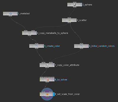
In a nutshell, I scatter metaballs over the surface of a sphere and update the color and scale of each metaball based on the solver from the earlier post. The guts of the project lives in a single geometry node and looks like:

Let's step through each node to see how the effect is achieved.

  1. The metaball node creates a single metaball. 
  2. The sphere node is the main "scaffold" over which the metaballs will be distributed.
  3. The scatter node distributes points across the main sphere.
  4. The copy_metaballs_to_sphere node creates multiple copies of the metaball at each of the points created by the scatter node. 
  5. By default, the copied metaballs don't have a color attribute, the create_color node creates that attribute.
  6. The initial_random_colors node assigns a random color to each point generated by the scatter node. 
  7. The copy_color_attribute node copies the random point colors to each metaball.
  8. The bz_solver node uses the VEX from Simulating Belousov-Zhabotinsky Reaction in Houdini to execute the simulation.
  9. Finally, the set_scale_from_color simply sets the x, y and z scales based on the color using the expression: (@Cd.r + @Cd.g)
Easy! 

Attributes are a core concept in Houdini, I'd thoroughly recommend watching Houdini Concepts Part 1 to learn more about them and the magical Attribute Copy node.  

Randomly Transforming Scattered Cones in Houdini

$
0
0
This post looks at a super simple Houdini project that scatters cones across the surface of a sphere and uses a Perlin noise function in a VEX wrangle node to randomly transform each cone. The resulting animation looks quite organic - maybe like a dancing sea urchin?

The network required for the effect only requires a handful of nodes, let's dive in an take a look:


  1. Much like my metaball morphogenesis project, this network requires a sphere to act as a scaffold for the overall effect. Its primitive type needs to be set to something other than primitive so that it outputs data for each vertex. Mine happens to be a polygon mesh.
  2. Even though the sphere node returns data for each vertex, it doesn't return normals. I need these to align the transform for each cone, hence the normal node.
  3. An additional scatter node jitters the positions of the points and allows me to control the exact count.
  4. The wrangle node adds some VEX to move each point based on a Perlin noise function.
  5. The cone, which will be distributed across the sphere's surface is simply a tube with one of its radii set to zero.
  6. Finally, the copy node copies and distributes the cone over the sphere at the locations of the transformed points.

The VEX in the wrangle node is pretty basic stuff. It uses the the position of each point and the time to generate a random value using the noise function. That value is multiplied by the normal value for each point to calculate its new position:


vector4 pos;pos.x = @P.x;
pos.y = @P.y;
pos.z = @P.z;
pos.w = @Time; 
vector rnd = noise(pos); 

@P.x += @N.x * rnd.z * 2;  
@P.y += @N.y * rnd.z * 2; 
@P.z += @N.z * rnd.z * 2; 
Adding a material with displacement gives a great result too:


Enjoy! 

Swarm Chemistry in SideFX Houdini

$
0
0


Hiroki Sayama's Swarm Chemistry is a model I've tinkered with and blogged about for years. Swarm chemistry simulates systems of heterogeneous particles each with genomes that describe simple kinetic rules such as separation and cohesion. As the simulation progresses, emergent phenomena such as mitosis and morphogenesis can be observed.

All of my previous implementations of swarm chemistry have been in two dimensions, but as part of my run-before-you-can-walk Houdini education, I thought I'd implement the maths in VEX and attempt a three dimensional Houdini version.

The results, I think, are pretty impressive. Rather than rendering plain particles, the system is rendered as metaballs and, combined with the additional dimension, it looks very organic.

Let's dive into my swarm chemistry node to see how it's all put together:


  1. The first node is a Point Generate which, as the name suggests, generate points. In my project, I create 7,500 points.
  2. I use a Color node to add a color attribute.
  3. The generated points are, by default, all at {0, 0, 0}, this Attribute Wrangle node places them randomly in a cube using:
    1. vector randomPosition = random(@ptnum);
    2. @P = -10 + (randomPosition * 20.0);
  4. The swarm chemistry code requires that each point has velocity and velocity2 attributes which are added in this Attribute Create node.
  5. The Solver node runs the swarm chemistry VEX which I'll describe later in this post.
  6. A Metaball node supplies the metaball geometry for the system.
  7. A Copy node copies a metaball to each point.
  8. Finally, an Attribute Transfer node transfers the point colors to the metaballs.
All simple stuff so far. The real work is done inside the solver which has an Attribute Wrangle attached to its "previous frame" DOP import. Grab yourself a cup of tea and I'll step through the VEX.

My first step is to figure out which of the three genomes will be used for the current point. This is done by using the modulo operator on the current point number. Using that value, I define the values for cohesion, alignment, separation, etc:

int index = @ptnum % 3;
float c1_cohesion = 0;
float c2_alignment = 0;
float c3_seperation = 0;
float c4_steering = 0;
float c5_paceKeeping = 0;
float radius = 0;
float normalSpeed = 0; 
if (index == 0)
{
    @Cd = {1, 0, 0};
    c1_cohesion = 73.63;
    c2_alignment = 0.95;
    c3_seperation = 3.2;
    c4_steering = 0.3;
    c5_paceKeeping = 0.35;    
    radius = 20;
    normalSpeed = 0.8; }
else if (index == 1)
{
    @Cd = {0, 1, 0};
    c1_cohesion = 53.63;
    c2_alignment = 0.75;
    c3_seperation = 2.9;
    c4_steering = 0.5;
    c5_paceKeeping = 0.3;    
    radius = 10;
    normalSpeed = 0.8;
}
else // index == 2
{
    @Cd = {0, 0, 1};
    c1_cohesion = 63.63;
    c2_alignment = 0.65;
    c3_seperation = 2.7;
    c4_steering = 0.2;
    c5_paceKeeping = 0.25;    
    radius = 25;
    normalSpeed = 2.8;
}
My next step is to iterate over each point's closest neighbors and start summing an accumulator with the distances of those neighbors multiplied by the genome's separation value:
int pointCloud = pcopen(0, "P", @P, radius, 1000); 
vector temp = {0, 0, 0}; 
while(pciterate(pointCloud)){    vector tmpP;    pcimport(pointCloud, "P", tmpP);        float dist = distance(@P, tmpP);         if (dist < 1)    {        dist = 1;     }        temp += (@P - tmpP) / (dist * c3_seperation); }
The average position and velocities of the neighboring points is calculated with pcfilter:
vector localCentre = pcfilter(pointCloud, "P"); vector localVelocity = pcfilter(pointCloud, "velocity"); 
A random steering value is added to the accumulator:
float r = random(@ptnum + @Time);if (r > c4_steering){    vector randSteer = (random(@ptnum * @Time) - 0.5) * 3;    temp += randSteer; }
The average position and velocity is also added to the accumulator, multiplied by the cohesion and alignment values of the genome:
temp += (localCentre - @P) * c1_cohesion;
temp += (localVelocity - v@velocity) * c2_alignment; 
Finally, the velocity is calculated based on the accumulator and the point's position is updated. Interestingly, I have to tell Houdini that my velocity and velocity2 attributes are vectors by prefixing them with a v (e.g. v@velocity):
v@velocity2 += temp * 0.1;
float d = length(v@velocity2); 
if (d < 0.1) {    d = 0.1; }
float accelerateMultiplier = 0; accelerateMultiplier = (normalSpeed - d) / d * c5_paceKeeping;
v@velocity2 += v@velocity2 * accelerateMultiplier ;
v@velocity = v@velocity2; 
@P += v@velocity * 0.1; 
Phew! 

Considering the work involved, Houdini renders the points pretty quickly - even in the UI of the app.

I hope you find this post useful, keep an eye out for more experiments in Houdini!

Creating a Swarm Chemistry Digital Asset in Houdini

$
0
0

My recent post, Swarm Chemistry in SideFX Houdini, illustrates an interesting effect, but tweaking the values in the swarm chemistry solver is a pain. What would be great is a user interface to vary the simulation parameters rather than having to edit the VEX by hand.

Luckily, Houdini offers two approaches to do this: HUD sliders and Digital Assets. In this post, I'll take a quick look at the latter.

A digital asset wraps up a network into a reusable node. The asset can expose a custom user interface containing sliders, buttons, color choosers and other UI controls.

The first step is to right-click the node you wish to convert to a digital asset and select "Create Digital Asset". After confirming the asset's name and location, you're presented with this slightly daunting dialog:


Here, you can define the UI controls you wish to create and the parameters they're bound to. In the figure above, the color of Genome One is selected and that refers to the color parameter, genomeOneColor.

For my swarm chemistry asset, my UI looks like:


Parameter values can be accessed inside the asset using the VEX channel functions such as ch() for floats and chv()for vectors. For example, the metaball checkbox at the top of the form is bound to a parameter named useMetaballs. A Switch node inside my network selects between the raw points or the copied metaballs, and its input parameter is controlled by an expression:


To access the asset's parameters in the VEX solver that is deeper in the network, I changed  the wrangle node's Evaluation Node Path property to the top level of the network. This means I don't need to worry about how deep the node and I can avoid prefixing multiple "../" to each parameter name. For example, I can access genome one's color and cohesion with this code:
@Cd = chv("genoneOneColor"); 
c1_cohesion = 100 * ch("cohesionOne");
Because the asset is saved locally, it's available to any other projects. My tab menu now has a new entry!


Powerful stuff! 

Using Houdini VOPs to Deform Geometry

$
0
0

Houdini VOPs, or VEX Operators, are networks that use a visual programming paradigm to create operators that can, for example, deform geometry, define material shaders or generate particle systems. There is a huge range of nodes available inside a VOP - everything from programming logic (e.g. conditionals and loops) to maths (e.g. dot and cross products) to domain specific operators for geometry and shaders.

My little demo project uses a VOP to deform the geometry of a sphere to look like an animated alien sea urchin. This geometry is then converted to a rigid body and the animation of its spiky protrudances moves it around the scene.

The main geometry node is pretty basic - a subdivided sphere feeding into an Attribute VOP:


It's inside the VOP that things get interesting.


  1. By default, a VOP is populated with a global parameters node. The position (P) and frame (Frame) parameters are used to drive the animation.
  2. The turbulent noise node is set to alligator noise and given an attenuation of 1.5.
  3. The output of the noise is used to displace each incoming point alongs its normal
  4. To color the geometry, the output of the turbulent noise will be multiplied by 25 - this parameter node contains that value.
  5. The multiply node multiplies the noise value by the parameter value.
  6. A color mix node interpolates between yellow and blue based on the multiplied noise value.
  7. Finally, the displaced point position and the color are piped into the VOP output.

I used the RBD Object shelf tool to convert my animated, displaced sphere into a rigid body. To have the physics working nicely with the animated geometry, "Use Deforming Geometry" is checked inside the RBD Object node inside the generated DOP Network.

And that's it! It actually looks as if VOPs are so powerful, one could avoid ever writing a line of VEX again - much like my Sweetcorn app!

Stripy Viscous Fluid Impacts in Houdini

$
0
0

My first Houdini blog post, Experimenting with Impacts in SideFX Houdini, discussed viscous fluid impacts. This post looks at how to add a little more detail to the fluid object - specifically, I wanted to add colored stripes to the fluid.

The source geometry for my FLIP object is a point cloud created from four boxes. The network starts with a single box which feeds into separate yellow and blue color nodes. In turn, these nodes create a point cloud using Points from Volume and the original geometry's color in copied to the points with an Attribute Copy. The two colored volumes are distributed using four transforms:


By adding jitter to the Points from Volume nodes, the network creates a point cloud with four colored stripes:


I used Houdini's shelf tools to create a viscous FLIP fluid from the point cloud, but changed the FLIP object's Input Type to Particle Field. To get my rigid bodies to interact with the fluid and experience drag, I changed the FLIP solver's Feedback Scale to 1.

The final step in creating the stripy liquid was to add an Attribute Transfer to the fluid surface geometry network automatically created by Houdini (I've colored it in yellow in the image below):


This transfers the color attribute from the points to the fluid geometry to give it the colored stripes.

The impacts objects are simple RBD objects given an initial velocity. 

Magic! 

Simulating Mitosis in Houdini

$
0
0


Here's a quick and easy way to create a procedural simulation of cell mitosis that, in my opinion, looks pretty impressive. 

The simulation is based on a point cloud which is wrangled inside a solver. My main network looks like:


  1. The initial point cloud is crated with a Point Generate. The video above starts with just ten points.
  2. The positions of the points are randomized with a Point Jitter.
  3. The Solver contains my mitosis simulation VEX which is described below.
  4. The final render uses metaballs with a mode of Threshold Radius. This mode helps reduce the "popping" effect caused by the creation of new points.
  5. ...which are copied to each point with a Copy node.

The real action takes place in an Attribute Wrangle inside the Solver. It begins with a few lines that separate each point by moving it away from the average position of its neighbors:


int pointCloud = pcopen(0, "P", @P, 1 , 50);
vector localCentre = pcfilter(pointCloud, "P");
vector v = set(@P.x - localCentre.x,
               @P.y - localCentre.y,
               @P.z - localCentre.z);
@P += v * 0.75; 
Each point is assigned an age attribute which is incremented by a small, random amount with each frame. If age is greater than one, I add a new point to the point cloud. The new point is slightly offset from the original point and the original point's age is reset to zero:


if (@age > 1) {
    vector randOffset;
 
    
randOffset.x = -0.01 + (noise(localCentre.x + $FF * @age) * 0.02);
    
randOffset.y = -0.01 + (noise(localCentre.y + $FF * @age) * 0.02);
    
randOffset.z = -0.01 + (noise(localCentre.z + $FF * @age) * 0.02);
 
    int newPoint = addpoint(geoself(), @P + 
randOffset);
 
    @age = 0;
}
else {
    @age += abs((random($FF * @ptnum)) * 0.05);
}
In previous projects, I've explicitly added attributes with an Attribute Create, however, it seems simply declaring age in the VEX adds it for me. 

In the video above, I used the stock "red velvet" material with some added noise for displacement and, of course, added depth-of-field for the final render.  

The default metaball mode, Field Radius, causes an apparent increase in radius when a new point is added to the cloud - as demonstrated in the video below:


Addendum


Here's an evolved example. In the VEX code, I've also added some code to add and increment a scale attribute:
if (@scale < 1) {
    @scale += 0.075;
}
The scale, which starts at zero, is inherited by the metaballs which prevents the "pop" effect when a new point is added.

The solver output is now plugged into two metaball nodes, but one of those metaball nodes acts as the input to a remesh and then onto a wireframe node:


This gives the effect of a collection of individual "cells" surrounded by a fine mesh - see above.

Creating a Geometric Structure from Mitosis

$
0
0

This post expands upon my previous post, Simulating Mitosis in Houdini. After watching Creating Points, Vertices & Primitives using Vex by Fifty50, I wondered what sort of structure my mitosis emulation would create if the generated points were joined to their parent by a connecting rod.

Thanks to the Fifty50 video, implementing this was a piece of cake. With each new point generated in my existing mitosis solver, I added code the create a new polyline primitive with two vertices - one based on the parent point and the other based on the newly generated point:


[...] 
int newPoint = addpoint(geoself(), @P + randOffest);      
int prim = addprim(geoself(), "polyline"); 
int vertex1 = addvertex(geoself(), prim, @ptnum); 
int vertex2 = addvertex(geoself(), prim, newPoint);  
[...]

With some additional code to limit the total number of child points each point can generate, the solver creates a series of connected lines:


To create the renderable geometry, I took the output from the solver and piped it into a PolyWire node to create the connecting rods, and a Copy node to place a sphere at each point. With that geometry, I generated a VDB volume which was smoothed and converted back to polygons:


The final result is a smooth mesh with no hard joints between the spheres and connecting rods. In my opinion, this gives a nicer look as the spheres divide that the metaballs I've used previously:


The video above shows the final render using the default silver material and an Environment Light added to the scene. Another win for Houdini!

More Chaos in Houdini: Simulating a Double Pendulum

$
0
0

I looked at creating strange attractors in Houdini recently and there's a more elegant solution over at Entagma. This post looks at an alternative way of modeling an attractor using SideFX Houdini with a double pendulum. As the pendulum swings, it generates a trail that describes its path through space.

The project can be split into two sections: modeling the double pendulum and creating the trail. 

Let's look at the double pendulum geometry first:

Creating a Double Pendulum

The double pendulum is made of two sections - the top and bottom. Each of these is constructed from two spheres and a connecting tube. These geometries are merged together and converted to a VDB. The VDB is smoothed and converted back to polygons. The bottom sphere of the top section has its bottom removed by a Cookie Boolean operator:


The final double pendulum looks like this - you can see how the bottom sphere has been clipped by the Cookie operator to look like a ball and socket joint:


I converted both sections into rigid bodies and added pin constraints in the AutoDopNetwork:


While top_pin_constraint doesn't have a goal object, bottom_pin_constraint uses the TOP geometry as its goal. This builds the hierarchy and, by giving both objects some initial angular velocity, the double pendulum starts happily swinging away.

Creating the Trail

The trail is built in a separate geometry node. It uses a Dop Import node to transform a sphere that follows the path taken by the bottom section. The Dop Import parents a single point which is fed into a Trail node. The result type for Trail is set to connect as polygons and converted to a VDB with a VDB from Polygons node:


Before the VDB is converted back to polygons, it's smoothed with a Gaussian VDB Smooth SDF node.

You can see a nicely rendered version above, here's a longer, 1,250 frame, OpenGL render:


Viewing all 257 articles
Browse latest View live